Visualization
We offer two routes to visualization. The first is using our own plotting routines, built atop Compose.jl. The second converts our trees to Phylo.jl trees, and plots with their Plots.jl recipes. The Compose, Plots, and Phylo dependencies are optional.
Example 1
using MolecularEvolution, Plots, Phylo

#First simulate a tree, and then Brownian motion:
tree = sim_tree(n = 20)
internal_message_init!(tree, GaussianPartition())
bm_model = BrownianMotion(0.0, 0.1)
sample_down!(tree, bm_model)

#We'll add the Gaussian means to the node_data dictionaries
for n in getnodelist(tree)
    n.node_data = Dict(["mu" => n.message[1].mean])
end

#Transducing the mol ev tree to a Phylo.jl tree
phylo_tree = get_phylo_tree(tree)

pl = plot(
    phylo_tree,
    showtips = true,
    tipfont = 6,
    marker_z = "mu",
    markeralpha = 0.5,
    line_z = "mu",
    linecolor = :darkrainbow,
    markersize = 4.0,
    markerstrokewidth = 0,
    margins = 1Plots.cm,
    linewidth = 1.5,
    markercolor = :darkrainbow,
    size = (500, 500),
)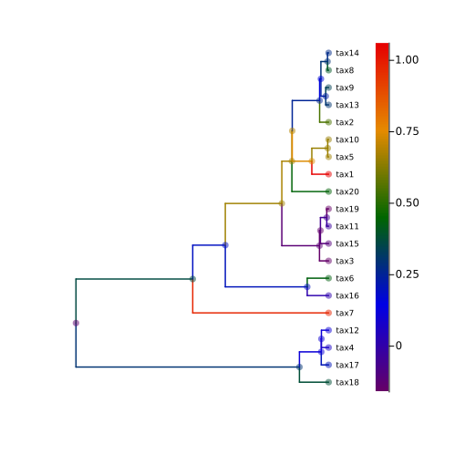
We also offer savefig_tweakSVG("simple_plot_example.svg", pl) for some post-processing tricks that improve the exported trees, like rounding line caps, and values_from_phylo_tree(phylo_tree,"mu") which can extract stored quantities in the right order for passing into eg. markersize options when plotting.
For a more comprehensive list of things you can do with Phylo.jl plots, please see their documentation.
Drawing trees with Compose.jl.
The Compose.jl in-house tree drawing offers extensive flexibility. Here is an example that plots a pie chart representing the marginal probability of each of the 4 possible nucleotides on all nodes on the tree:
using MolecularEvolution, Compose

tree = sim_tree(40, 1000.0, 0.005, mutation_rate = 0.001)
model = DiagonalizedCTMC(reversibleQ(ones(6), ones(4) ./ 4))
internal_message_init!(tree, NucleotidePartition(ones(4) ./ 4, 1))
sample_down!(tree, model)
d = marginal_state_dict(tree, model);compose_dict = Dict()
for n in getnodelist(tree)
compose_dict[n] =
(x, y) -> pie_chart(x, y, d[n][1].state[:, 1], size = 0.02, opacity = 0.75)
end
img = tree_draw(tree,draw_labels = false, line_width = 0.5mm, compose_dict = compose_dict)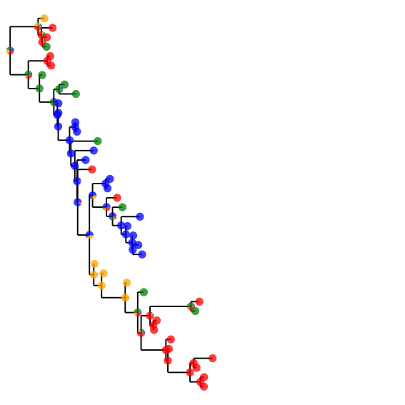
This can then be exported with:
savefig_tweakSVG("piechart_tree.svg",img);Multiple trees
Doesn't require Phylo.jl. Query trees can be plotted against a reference tree with plot_multiple_trees. This can be useful, for instance, when we've sampled trees with metropolis_sample.
using MolecularEvolution, Plots

tree = sim_tree(10, 1, 1)
nodelist = getnodelist(tree); mean = sum([n.branchlength for n in nodelist]) / length(nodelist)
rparams(n::Int) = MolecularEvolution.sum2one(rand(n))
model = DiagonalizedCTMC(reversibleQ(ones(6) ./ (6 * mean), rparams(4)))
internal_message_init!(tree, NucleotidePartition(ones(4) ./ 4, 100))
sample_down!(tree, model)
@time trees, LLs = metropolis_sample(tree, [model], 300, collect_LLs=true);
4.792793 seconds (18.42 M allocations: 1.383 GiB, 3.73% gc time, 36.33% compilation time)We'll use the HIPSTR tree as reference
reference = HIPSTR(trees);
plot_multiple_trees(trees, reference)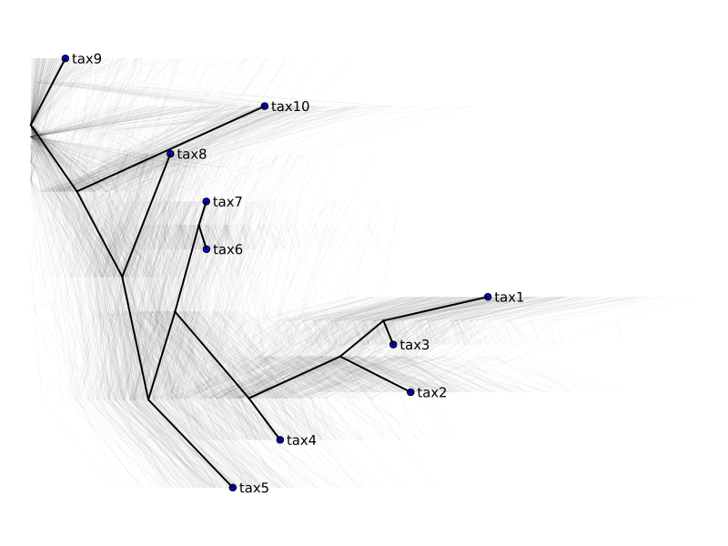
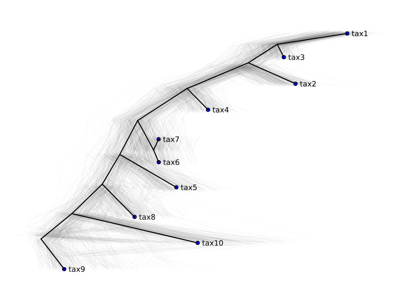
We can pass in a weight function to fit query trees against reference in a weighted least squares fashion with a location and scale parameter.
Note
If we don't want to scale the query trees, we must disable it with opt_scale = false.
plot_multiple_trees(
    trees,
    reference,
    y_jitter = 0.05,
    weight_fn = n::FelNode ->
       ifelse(MolecularEvolution.isroot(n) || isleafnode(n), 1.0, 0.0)
)
Functions
MolecularEvolution.get_phylo_tree Function
get_phylo_tree(molev_root::FelNode; data_function = (x -> Tuple{String,Float64}[]))Converts a FelNode tree to a Phylo tree. The data_function should return a list of tuples of the form (key, value) to be added to the Phylo tree data Dictionary. Any key/value pairs on the FelNode node_data Dict will also be added to the Phylo tree.
MolecularEvolution.values_from_phylo_tree Function
values_from_phylo_tree(phylo_tree, key)

Returns a list of values from the given key in the nodes of the phylo_tree, in an order that is somehow compatible with the order the nodes get plotted in.MolecularEvolution.savefig_tweakSVG Function
savefig_tweakSVG(fname, plot::Plots.Plot; hack_bounding_box = true, new_viewbox = nothing, linecap_round = true)Note: Might only work if you're using the GR backend!! Saves a figure created using the Phylo Plots recipe, but tweaks the SVG after export. new_viewbox needs to be an array of 4 numbers, typically starting at [0 0 plot_width*4 plot_height*4] but this lets you add shifts, in case the plot is getting cut off.
eg. savefig_tweakSVG("export.svg",pl, new_viewbox = [-100, -100, 3000, 4500])
savefig_tweakSVG(fname, plot::Context; width = 10cm, height = 10cm, linecap_round = true, white_background = true)Saves a figure created using the Compose approach, but tweaks the SVG after export.
eg. savefig_tweakSVG("export.svg",pl)
MolecularEvolution.tree_draw Function
tree_draw(tree::FelNode;
    canvas_width = 15cm, canvas_height = 15cm,
    stretch_for_labels = 2.0, draw_labels = true,
    line_width = 0.1mm, font_size = 4pt,
    min_dot_size = 0.00, max_dot_size = 0.01,
    line_opacity = 1.0,
    dot_opacity = 1.0,
    name_opacity = 1.0,
    horizontal = true,
    dot_size_dict = Dict(), dot_size_default = 0.0,
    dot_color_dict = Dict(), dot_color_default = "black",
    line_color_dict = Dict(), line_color_default = "black",
    label_color_dict = Dict(), label_color_default = "black",
    nodelabel_dict = Dict(),compose_dict = Dict()
    )
Draws a tree with a number of self-explanatory options. Dictionaries that map a node to a color/size are used to control per-node plotting options. compose_dict must be a FelNode->function(x,y) dictionary that returns a compose() struct.
Example using compose_dict
str_tree = "(((((tax24:0.09731668728575642,(tax22:0.08792233964843627,tax18:0.9210388482867483):0.3200367900275155):0.6948314526087965,(tax13:1.9977212308725611,(tax15:0.4290074347886068,(tax17:0.32928401808187824,(tax12:0.3860215462534818,tax16:0.2197134841232339):0.1399122681886174):0.05744611946245004):1.4686085778061146):0.20724159879522402):0.4539334554156126,tax28:0.4885576926440158):0.002162260013924424,tax26:0.9451873777301325):3.8695419798779387,((tax29:0.10062813251515536,tax27:0.27653633028085006):0.04262434258357507,(tax25:0.009345653929737636,((tax23:0.015832941547076644,(tax20:0.5550597590956172,((tax8:0.6649025646927402,tax9:0.358506423199849):0.1439516404012261,tax11:0.01995439013213013):1.155181296134081):0.17930021667907567):0.10906638146207207,((((((tax6:0.013708993438720255,tax5:0.061144001556547097):0.1395453591567641,tax3:0.4713722705245479):0.07432598428904214,tax1:0.5993347898257291):1.0588025698844894,(tax10:0.13109032492533992,(tax4:0.8517302241963356,(tax2:0.8481963081549965,tax7:0.23754095940676642):0.2394313086297733):0.43596704123297675):0.08774657269409454):0.9345533723114966,(tax14:0.7089558245245173,tax19:0.444897137240675):0.08657675809803095):0.01632062723968511,tax21:0.029535281963725537):0.49502691718938285):0.25829576024240986):0.7339777396780424):4.148878039524972):0.0"
newt = gettreefromnewick(str_tree, FelNode)
ladderize!(newt)
compose_dict = Dict()
for n in getleaflist(newt)
    #Replace the rand(4) with the frequencies you actually want.
    compose_dict[n] = (x,y)->pie_chart(x,y,MolecularEvolution.sum2one(rand(4)),size = 0.03)
end
tree_draw(newt,draw_labels = false,line_width = 0.5mm, compose_dict = compose_dict)


img = tree_draw(tree)
img |> SVG("imgout.svg",10cm, 10cm)
OR
using Cairo
img |> PDF("imgout.pdf",10cm, 10cm)MolecularEvolution.plot_multiple_trees Function
plot_multiple_trees(trees, inf_tree; <keyword arguments>)Plots multiple phylogenetic trees against a reference tree, inf_tree. For each tree in trees, a linear Weighted Least Squares (WLS) problem (parameterized by the weight_fn keyword) is solved for the x-positions of the matching nodes between inf_tree and tree.
Keyword Arguments
node_size=4: the size of the nodes in the plot.line_width=0.5: the width of the branches fromtrees.font_size=10: the font size for the leaf labels.margin=1.5: the margin between a leaf node and its label.line_alpha=0.05: the transparency level of the branches fromtrees.y_jitter=0.0: the standard deviation of the noise in the y-coordinate.weight_fn=n::FelNode -> ifelse(isroot(n), 1.0, 0.0)): a function that assigns a weight to a node for the WLS problem.opt_scale=true: whether to include a scaling parameter for the WLS problem.
MolecularEvolution.HIPSTR Function
HIPSTR(trees::Vector{FelNode}; set_branchlengths = true)Construct a Highest Independent Posterior Subtree Reconstruction (HIPSTR) tree from a collection of trees.
Returns a single FelNode representing the HIPSTR consensus tree.
If
set_branchlengths = true, the branch length of a node in the HIPSTR tree will be set to the mean branch length of all nodes from the input trees that have the same clade. (By the same clade, we mean that the set of leaves below the node is the same.) Otherwise, the root branch length is 0.0 and the rest 1.0.If
getcred = true, then(hipstr_tree, node2logcred)is returned, wherenode2logcredis a dictionary mapping eachFelNodein thehipstr_treeto its log-domain credibility score.
Source: https://www.biorxiv.org/content/10.1101/2024.12.08.627395v1.full.pdf
sourceThis page was generated using Literate.jl.